Co-localization is a powerful concept in fluorescence microscopy that helps scientists understand whether two or more molecules occupy the same location within a cell, tissue, or subcellular structure. When multiple fluorophores emit light from overlapping regions, their signals combine in the image, revealing potential molecular interaction
What is Co-Localization?
In biological terms, co-localization occurs when molecules bind to the same receptor or exist in very close proximity. Digitally, it’s observed as pixels in an image containing contributions from more than one fluorophore for example, green-emitting Alexa Fluor 488 and red-emitting Alexa Fluor 568 creating yellow pixels where their signals overlap.
Confocal microscopy captures images as voxels, three-dimensional pixels representing a volume in the specimen. Each voxel’s size depends on the objective’s numerical aperture, illumination wavelength, and pinhole diameter, making confocal imaging precise for co-localization studies.
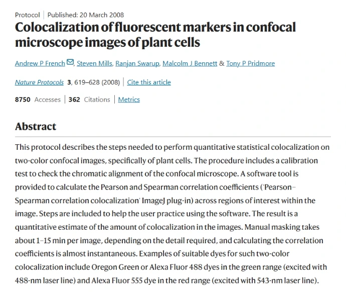
For more detailed information, you can read the article titled
“Colocalization of Fluorescent Markers in Confocal Microscope Images of Plant Cells.”
Choosing the Right Fluorophores
Accurate co-localization requires careful selection of fluorophores with well-separated emission spectra. Overlapping spectra can cause bleed-through artifacts, producing false co-localization signals. For instance:
Alexa Fluor 488 + Alexa Fluor 555: Moderate spectral overlap; may need multitracking to avoid bleed-through.
Alexa Fluor 488 + Alexa Fluor 633 or 647: Minimal overlap; ideal for accurate co-localization.
Modern synthetic fluorophores like the Alexa Fluor and Cy series are bright, stable, and available in a wide range of wavelengths, reducing artifacts common with traditional dyes such as fluorescein and rhodamine.
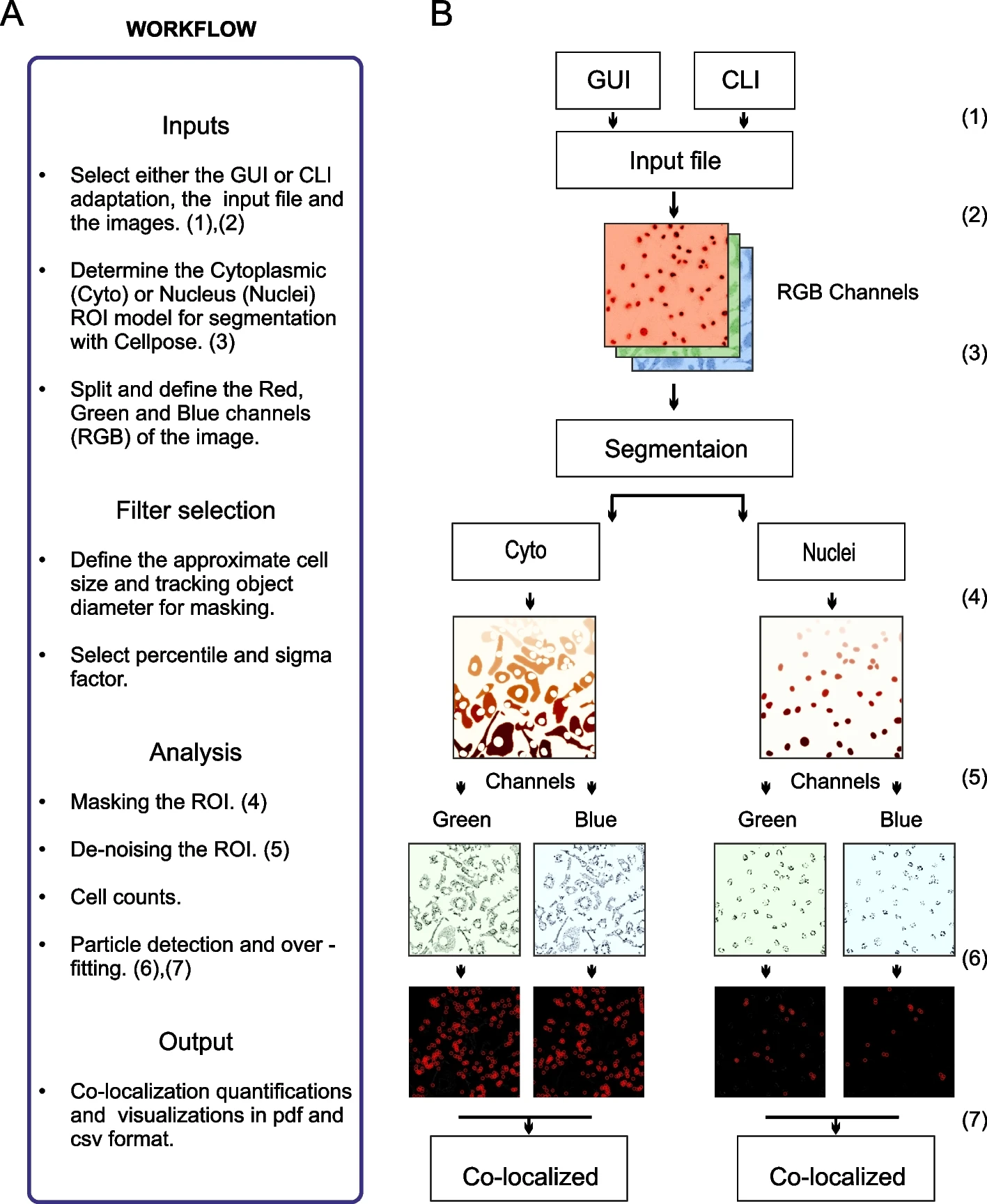
Figure: SpotitPy: Workflow and Design for Automated Particle Tracking and Co-localization
This figure provides an overview of the SpotitPy software workflow implemented in Python. Users can choose either the GUI or CLI interface (1) and supply input images meeting the required specifications (2). Experimental parameters are set next, including segmentation model selection and threshold definition (3). The software then identifies cellular compartments, generates ROI masks (4), de-noises images (5), estimates cell counts, and performs particle tracking in each channel. Detected particles across channels are then analyzed to determine co-localization (6–7). All outputs are compiled into data files, while visualizations of each step are generated using Matplotlib (B), with numerical identifiers corresponding to workflow stages.
Imaging and Software Analysis
Confocal microscopes capture optical sections to minimize vertical overlap in thicker specimens. For thinner samples (<5 µm), widefield fluorescence may suffice, but confocal or multiphoton imaging is preferred for thick tissues.
Software tools allow quantitative co-localization analysis by comparing pixel intensity between channels. Scatterplots (fluorograms) graph intensities of two channels for each pixel:
Pure single-color pixels cluster near the axes.
Co-localized pixels appear along the diagonal (x = y), often as yellow or orange.
Common metrics include:
Pearson’s correlation coefficient (R) – measures similarity in spatial patterns.
Overlap coefficient (R, k, m, M values) – quantifies the fraction of co-localized fluorescence, accounting for intensity differences.
These coefficients help evaluate molecular interactions while controlling for background, photobleaching, and intensity variations.
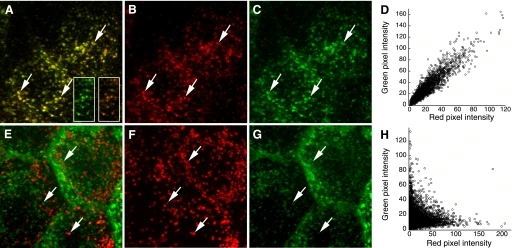
Figure: Colocalization Analysis of Endocytic Probes in MDCK Cells
This figure illustrates colocalization of endocytic markers in Madin Darby Canine Kidney (MDCK) cells. (A) Maximum projection of a cell volume after incubation with transferrin conjugated to Texas Red (B) and Alexa 488 (C); arrows highlight endosomes containing both probes. (D) Scatterplot of red versus green pixel intensities from the cells in (A) quantifies colocalization. (E) Maximum projection following incubation with Texas Red-dextran (F) and Alexa 488-transferrin (G), with arrows indicating lysosomes containing Texas Red-dextran. (H) Corresponding scatterplot shows pixel intensity correlation, providing quantitative assessment of probe overlap.
Practical Tips for Co-Localization
Pseudocolor images help visualize overlap: green + red = yellow; blue combinations are less intuitive for the human eye.
Adjust gain and offset carefully to avoid misinterpretation of merged channels.
Ratio imaging or multitracking can distinguish true co-localization from partial overlaps.
Always verify with controls before drawing conclusions about molecular interactions.
Avoiding Artifacts
Artifacts can mislead co-localization studies. Major sources include:
Spectral bleed-through – emission from one fluorophore detected in another channel.
Autofluorescence – inherent tissue fluorescence can mimic co-localization.
Non-specific staining – antibodies or fluorophores binding off-target.
FRET effects – energy transfer between closely spaced fluorophores may alter signal intensity.
Best practices to minimize artifacts:
Use fluorophores with widely separated emission spectra.
Optimize antibody and fluorophore specificity.
Perform single-labeled and unstained control experiments.
Use sequential scanning in confocal microscopy to collect each fluorophore separately.
Employ narrow bandpass emission filters and high-quality apochromatic objectives to reduce chromatic aberration.

In the book Cell Imaging (pages 97–109), the article "Colocalization Analysis in Fluorescence Microscopy" provides a clear explanation of this technique."
Conclusion
Fluorophore co-localization in confocal microscopy is a key tool for visualizing molecular interactions. Success depends on:
Careful fluorophore selection and sample preparation
Optimized microscope configuration
Robust image acquisition and software analysis
When executed correctly, co-localization studies reveal critical insights into cell signaling, protein interactions, and subcellular architecture—unlocking the hidden connections in biological systems.
